In Part 1, I made the case that, for regular NHL defencemen, On-Ice Save Percentage (OISV%) was not independent of their performance and that those defencemen who leak high quality scoring chances against (Chance Quality Against) have their goalies save a lower percent of shots while they are on the ice. I also pointed out that Edmonton Oilers defenceman Caleb Jones is a player who has both a low OISV% and a high average Chance Quality Against, and that the former is likely at least partially attributable to the latter. In Part 2, I’m trying to tackle the question: How many goals did a poor OISV% add to Jones’s total this year? We know he got a relatively low save percentage when he was on the ice, but how much lower than we should have expected? To answer these questions, I will fit a linear model based on his performance (using the metric I introduced in Part 1) and another metric to help us make sense of the numbers. And that metric is…
Goaltending
The biggest hole in the claims I made in part 1 is that never did I include any measure of the quality of a team’s goaltending. We were predicting OISV% independent of goaltending, which is an unusual thing to try to do. In addition to making it easier to understand the relationship between Chance Quality Against and OISV%, including a measure of goaltending ability allows us to better evaluate how good a predictor Chance Quality Against is of OISV%. Remember that the correlation between the two was around -.3 (and thus Chance Quality Against alone explained about 8% of the variance in OISV%), which is a little bit tough to evaluate in isolation. Maybe it’s not very good (it’s not a large correlation). However, if the quality of the goaltending is explaining most of what’s left, then maybe that high of a correlation actually is pretty good. So, let’s include the goalie’s save percentage and see what happens.
This presents a bit of a conundrum: how? Not all defencemen played in every game, and not always in front of the same goalie. Some were traded midseason, so which team’s save percentage to give them? In lieu of painstakingly coding which games were played by which defensemen in front of which goalies on which teams, I’ve taken a bit of a shortcut here and made the assumption that players generally play more games for whichever team they start the season with. In addition, I’ve collapsed across all goalies that played for a team in a given season. So, I’ve attached to each player the season average 5v5 save percentage of the team they started the season with. Presumably, this causes some real but small inaccuracy in the model.
The Model
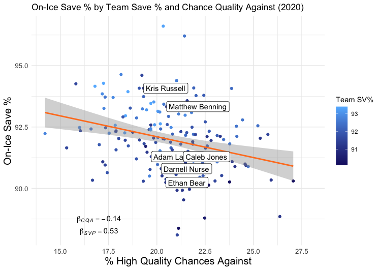
I fit a regression model with two predictors (Team SV% and Chance Quality Against, which as a reminder is High Danger Chances Against/Total Chances Against) and one response variable (OISV%) for each of the past two years. This is a very, very simple model because it only contains two predictor variables. It is not meant to be the strongest model I could come up with, but rather one that is easy enough to understand. For both 2020 and 2021, both variables were significant predictors of OISV%. In other words, both Team SV% and Chance Quality Against improve our ability to predict OISV%.
For 2020:
For 2021:
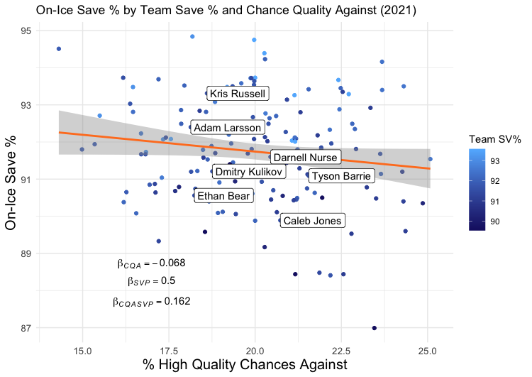
You’ll notice these are the same scatterplots as shown in Part 1, but with the added dimension of Team Save %, which can be seen here as a blue gradient (the orange and blue colour scheme was intentional).
As for how well these two variables together explain OISV%, the R2 of these models are 0.34 and 0.31, respectively. This means that, where in Part 1 we could explain about 8% of the variance in OISV% with just Chance Quality Against, now we can explain almost 35%. In other words, given hockey is a sport with lots of noise and randomness, and given we’ve only included two variables in our model, we’ve got a pretty decent (but by no means great) model of what goes into OISV% – goalie quality, and Chance Quality Against.
What Can the Model Tell Us about Caleb Jones?
It feels like I haven’t mentioned Caleb Jones in forever. The benefit of having a passable model is that we can plug Caleb Jones’s numbers in and get a predicted OISV% for this past season, given both the quality of chances against when he’s on the ice and the year-average of Oilers’ goaltending. We already know he got a lower-than-expected OISV% this season, but by how much? If a lot, maybe it’s worth banking on the randomness turning in his favour next year, even if he performs only equally as well as this year. If he underperformed only a little, it would be unreasonable to expect a large jump in his on-ice goal numbers unless he’s able to make large strides in limiting high-danger chances (remember from part 1 this is a measure that has some stability over years) and unless the team is able to get consistently better 5v5 goaltending. So, what is Jones’s predicted (by the model) OISV%? 91.28%, or about 1.3% higher than he got this season. If you don’t think that sounds like a lot, you’re right. When applied to the shots faced with Jones on the ice this past season (178), that’s a predicted 15.52 on-ice goals against. About two and a half less than reality. His corresponding GF% if nothing changed offensively would be 41.5%.
So, how much did On-Ice Save Percentage hurt Caleb Jones’s season? When you factor in only a measure of the opposition’s chance quality with him on the ice and the season average of his goalies’ performance, about two and a half goals. Maybe he takes a large step forward next season (25-year-old defencemen have been known to do that), and maybe the randomness that is hockey shaves a couple goals off his total, but you probably cannot expect the randomness alone to make Caleb Jones a positive impact 5v5 player. In other words, this year Caleb Jones was not a positive impact 5v5 player hidden by poor goaltending or bad puck luck behind him.
Some Limitations
There are, of course, some limitations to this analysis. One is that the model is not fantastic, but one wouldn’t expect it to be fantastic with only two input variables. Maybe someday I’ll try to build a better model with more input variables and see if anything changes, but today is not that day. Besides, my hunch is that, if anything, more input variables will be less-than-friendly to Jones. Do you remember in Part 1 when I pointed out that a certain type of defenceman (Kris Russell, Matt Benning, Adam Larsson) outperformed the model while others (Ethan Bear, Jones) underperformed? My suspicion is that there is some quantifiable reason for this, related to play style or something similar, and if you could find it and input it into the model, his predicted OISV% becomes even closer to his actual OISV%. Another limitation is that perhaps I haven’t chosen an optimal measure of either goalie quality (team save percentage) or Chance Quality Against, and there’s some resulting noise. Yet another is that perhaps the relationships change when you include more or fewer defencemen (or some, like Oscar Klefbom, who played in one but not both seasons), and my selection criteria were problematic.
___________________________________________________________
You can find me on Twitter @OilersRational. I’ve made my code and the data I used (adapted from Natural Stat Trick) available here if you want to try running this analysis for yourself or tweaking parts of it. I’m also available for help if you want to get into analyzing data but don’t know where to start.
Add The Sports Daily to your Google News Feed!