I have to apologize right up front for today’s column: not for the content, which I think is pretty good, but for the fact that it’s an old article I wrote for my other blog back at the end of June. I just started a new job today, and am in the middle of getting a new apartment, so I can’t devote the time to writing I’d like. In the meantime, hopefully most of you haven’t seen this before. The basic bent was to attempt to identify a few of the causes of a team over- or under-performing their Pythagorean predicted record (here’s a good explanation of Bill James’ Pythagorean Win Theorem, for those of you that might be unfamiliar with it; the article also includes Clay Davenport’s revisions to the formula). Hopefully this might spark a little discussion; there have been a lot of differing explanations for Pythagorean differentials, and this certainly doesn’t answer any questions. Instead, I hoped it would just introduce a few ways to look at the problem, and test some of the hypotheses floating around. Enjoy.
—-
For the last few weeks, I’ve been looking at Pythagorean Win % differentials, trying to figure out exactly what causes them – whether they’re predictable or random, whether they are related more to quantifiable team performance or to chance and luck. I wanted to take a look at this after watching the Washington Nationals continue to lead their division, despite having allowed more runs than they’ve scored. Is there something we can point to historically that might suggest why the Nats have been able to keep a winning record despite being outscored by their opponents? That’s sort of the inspiration for his post.
Background
This is old hat to many people, but for those of you that don’t know what the hell I’m talking about, here’s a quick background on the Pythagorean Win Theorem. Devised by Bill James in the 1980’s, the goal of the Theorem was to be able to predict a team’s W-L record based on how many runs it scored and how many it allowed; it’s called the Pythagorean Theorem because the actual formula bears a resemblance to the Pythagorean Theorem for determining the length of the hypotenuse of a right triangle. According to James, the square of runs scored divided by the sum of the squares of runs scored and runs allowed provides you with a percentage that comes remarkably close in virtually every case to the actual winning percentage of the team. To put it simply, if a team were to score exactly as many runs as their opponents, one would assume their record to be very close to .500. The more runs a team scores, the higher their winning percentage would logically become. James’ formula allowed people to look at that relationship concretely. These calculations are sometimes exactly equal, providing a W-L record that matches what a team actually did. Other times, they are slightly off; nevertheless, the majority of results are within 3 games of the actual W-L record, which is a fairly impressive correlation.
This study is concerned with the differential between teams’ actual winning percentage – the percentage of wins to total games that a team actually recorded – and its Pythagorean Win %, based on James’ theorem. I’m looking for trends that help explain why some teams perform better or worse than their Pythagorean; is it luck and chance, or are there certain aspects of team performance that impact the difference? For example, does a team that outperforms its expectations have a better offense, or bullpen? Are they better at stealing bases, or fielding? These are the things I’ll look at in more detail below.
Methodology
The data here was compiled for all teams from 2000-2004. Only teams between 6 games above and 6 games below were charted, as teams above or below that span are few, and tend to skew the data. Still, of the 150 team performances over those 5 years, 137 remain chartable.
To go about examining Pythagorean Win Differentials, I first broke down the potential variables involved. On a team level, these included Runs Scored, Runs Allowed, Win Percentage in 1 run games, Win Percentage in blowout games (defined here as games in which the winner and loser were separated by 7 or more runs), and a comparison number: Win % in 1 run and blowout games minus the actual team Win %. This latter allowed me to look at teams that were both better and worse than their actual record in these games.
Then I looked at individual aspects of a team’s performance: offensively, team OBP, SLG, and OPS; Starter and Reliever K/9, OPS Allowed, and ERA; so-called “small ball” numbers such as SB success rate, sacrifice bunts, and strikeouts (as a quick way to look at ability to put the ball in play); and fielding stats (fielding percentage, defensive range factor, and defensive zone ratings). Fielding stats were only available for the years 2002-2004.
Given the variability in the data by year, I placed each category on a 100-point scale (so that in 2002, for example, the Yankees, who led the majors in OBP, have a 100% OBP%, while the Mets – 21st in OBP – have a 40.7% OBP% and so on). This allows me to compare percentages of the largest variable in each character, and equalizes the numbers over the 5 year span.
Finally, I scored the data by differential, and charted each variable by differential, so we can visually see how each category responds to the change in differential.
The Charts
To present this data, and to get a good look at how much deviation there is in the data, I’ve employed Excel charts, with Pythagorean differentials as the X axis and the variables as the Y axes. In addition, I’ve added two different trend lines; the first is linear, a straight line that approximates the data trend, but suffers in that it tends to lose more of the variation in somewhat non-linear data. The second is a polynomial line, which reacts to changes and deviations in the data. The closer these two lines are to each other, the more certain we can be in the data. Furthermore, I’ve provided the R-squared numbers for each: these are located in the upper-right hand corner of each chart. The higher these numbers are – the closer they are to 1 – the less deviation there is in the data. So, a completely horizontal trend line with an R-squared of 1 means that there is no trending, but a definite correlation, whereas a horizontal trend line with an R-squared of .0001 means that there is no trending and no correlation (that the data is totally random and not indicative of any real relationship between the X and Y axes). Got that? Good.
The Assumptions
I tried to go into this with no assumptions as to the results; that’s a good thing, as many of the ones I would have had ended up disproved. Some of the basic assumptions regarding Pythagorean differentials are that teams that over-perform have a better bullpen (and therefore don’t lose close games as much), or play better small-ball (manufacturing runs when needed to win close ones), etc. Mostly, the assumption is that teams that do better in close games will outperform their Pythagorean, which makes logical sense (for example, winning 6 straight games by a score of 2-1 gives you a Pythagorean W-L of .667, or 4 wins, 2 losses. Since you won all six games, you’ve outperformed your Pythagorean in those games by 2). Another assumption is that a large number of blowouts won will have the opposite effect. Since winning blowouts requires a high scoring offense, one logical conclusion would be that scoring a lot of runs would actually decrease a team’s differential. But, regardless of the assumptions, chances are something in here negates one or more of them. So, let’s look at the actual data.
The Variables
First, I examined the most basic stats: runs scored and runs allowed. Obviously, runs scored and run allowed affect the Pythagorean win percentage (PW%) itself, but do they have any correlation with differentials?
(All of these charts are linked to larger versions in which they’re cleaner and clearer)
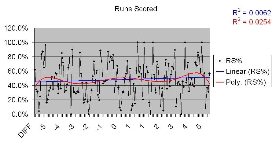
As you can see in this chart, there is basically no correlation between a team’s runs scored and its PW%. This is interesting to note, given that assumption that a strong offense wins more blowouts, and therefore has a negatively skewed Pythagorean.
Now, the data for Runs Allowed:
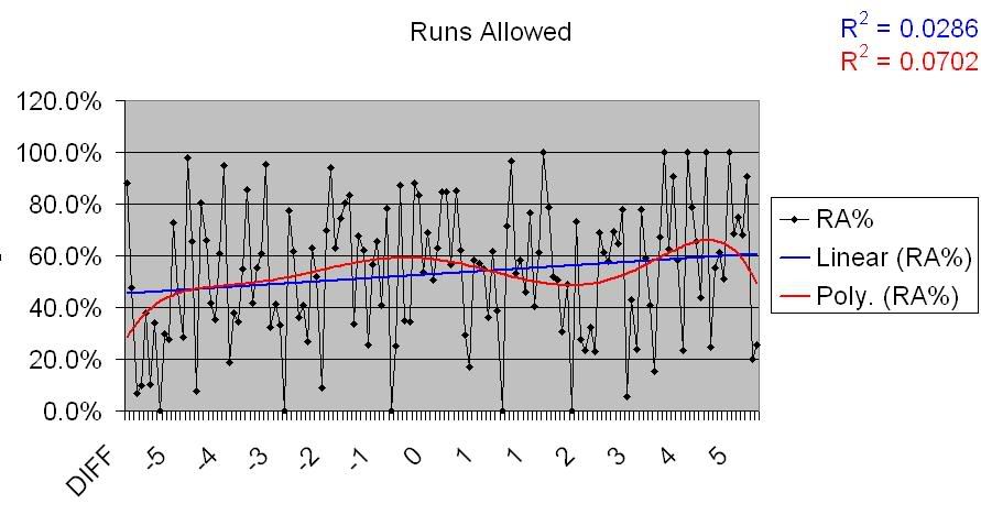
So, nothing groundbreaking. Maybe a slight uptick, but nothing that’s at all obvious. However, let’s take a closer look at this chart. First, we’ll take a look at the teams that over-perform their Pythagorean, by RA.
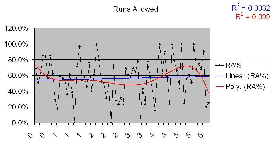
There’s virtually no correlation there. So, the number of runs a team allows has no bearing on whether they will overperform their PW%, at least not on a general level. What about those that underperform?
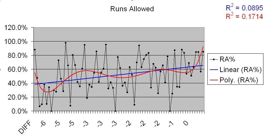
Now that’s interesting. There is a very visible correlation there; not absolute, but enough of one to take note. Given that this has popped up with Runs Allowed, we’ll take a look at the pitching numbers a little later and see if that carries through.
First, though, let’s see if the larger assumptions – that a good record in 1 run games positively impacts the differential, and a good record in blowout games negatively impacts it – hold true.
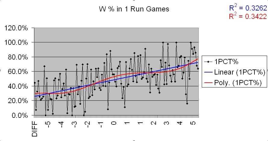
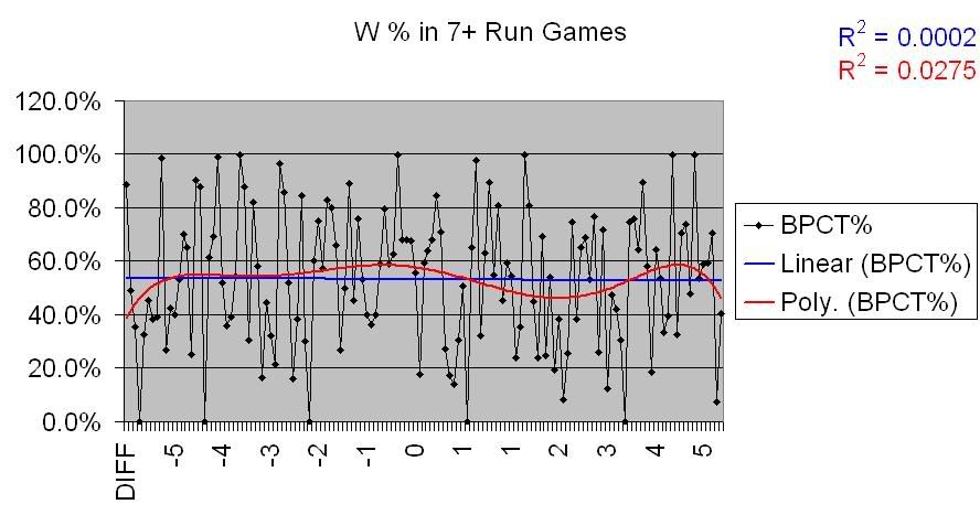
In the first chart, there’s an unmistakable correlation. Teams that do better in 1 run games over the course of a season outperform their Pythagoreans, definitively. However, the chart for blowout games shows the opposite; there is effectively no correlation between win % in blowouts and a Pythagorean differential.
But win percentages in those games don’t tell the whole story. A team that posts a .600 win percentage in 1 run games has performed better in them, but if that team holds a .600 win percentage overall, the result in the 1 run games is predictable. The same holds true for blowouts. So, let’s look at the results for close and blowout games in relation to the teams’ actual win-loss records:
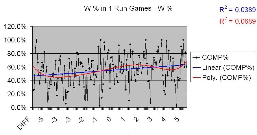
These figures are simple subtraction; the percentage above or below the actual W-L that teams post in close and blowout games. And, indeed, there are definite changes here. For 1 run games, the amount a team’s W-L varies from their actual record has a slight correlation with their Pythagorean differential. For blowout games, however, it’s much more defined; teams that lose a higher percentage of their blowout games than they do their actual W-L overperform their Pythagorean significantly. This difference is important, and I’ll talk about its importance towards the end of this piece.
So, now let’s look at some of the components of team performance, and see which ones hold correlations.
First, the offense. I’ve used only two numbers here; a team’s on-base percentage and its slugging percentage. Getting baserunners on and collecting a large number of total bases are the two most important things an offense can do, so these seem like reasonable choices; obviously there are other categories I could have – and possibly should have – looked at, but I’m operating under the assumption that any correlation between offense and Pythagorean differential will show itself in these two numbers.
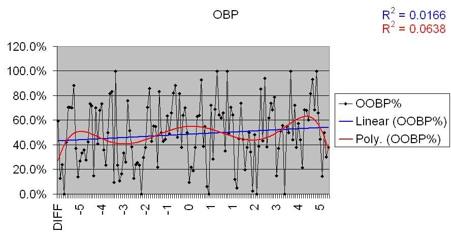
There’s maybe a very slight correlation there, but nothing large or certain enough to come to any conclusions about; much of that could be random fluctuation, and the deviation in the data points are simply too large to put any stock in them. Combine that with what we learned above regarding Runs Scored, for which there was no correlation, and we can tentatively say that there’s no correlation between raw offensive output and Pythagorean differentials.
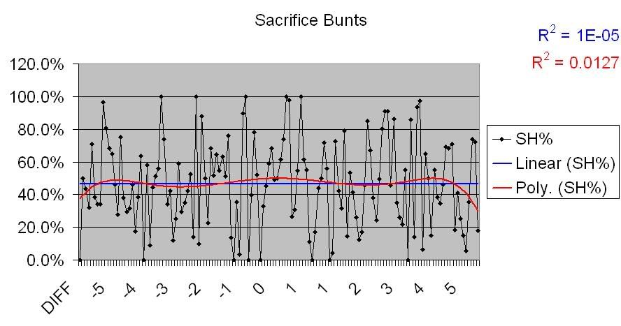
But how about the smaller aspects of an offense? By this, I mean the things that are commonly called ‘small-ball’: moving runners along, bunting, stealing bases. When discussing close games, and teams’ performance in them, many commentators claim that this happens because teams ‘do the little things’ right. So, let’s see if that olds true. We’ve seen that there is a very strong correlation between 1 run games and Pythagorean differential, so if small-ball does impact the former, it should show at least some correlation in the latter.
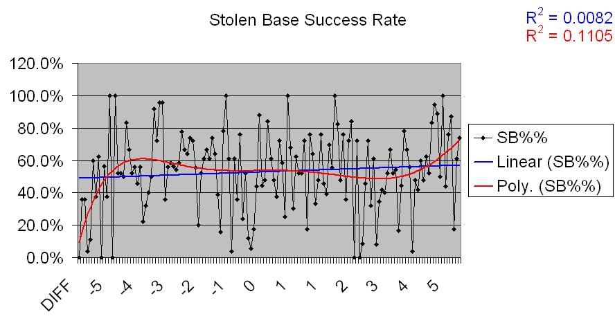
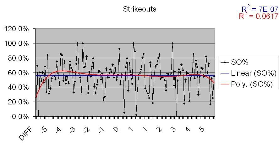
I wanted to use Productive Outs in this section, but what unable to find full data for the years involved, so instead I’ looking at strikeouts, the theory being that teams that strikeout more fail to move runners along, fail to put the ball in play, etc. It’s been fairly conclusively shown that high K rates come with high walk rates, and therefore low contact rates, so this seems at least a reasonable conclusion.
As we can see from this data, there is absolutely no correlation. The data is completely divergent, as you can see from the linear trendlines in those charts. From this, we ca very nearly conclusively say that small-ball and “doing the little things” have nothing at all to do with a team’s Pythagorean differential (That’s not to say these thing sdon’t mean anything in general, of course; just to say that they don’t have anything to do with overperforming the RS/RA of a team. One could also extrapolate from that that these things don’t have much impact on 1-run games, as is commonly thought.)
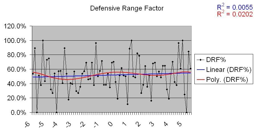
Defense is related to these findings, but on the other side; a defense ‘does the little things’ in terms of runs allowed. Now, the fielding data that I was looking at, aside from Fielding Percentage, only covered from 2002-2004, so I can’t say anything really conclusive about it. What I can say is that the data that exists doesn’t show any sort of correlation, but the lack of wider sample makes m hesitate to say this with any certainty. That having been said, here are the charts for the data that does exist.
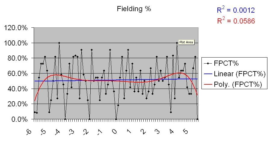
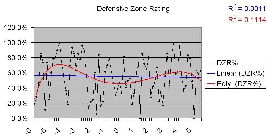
So, again with the caveat that there’s not as much data here as there is for other categories, it would appear that there’s no correlation present between fielding and Pythagorean differentials.
So, now we come to the last aspect of a team’s performance that I’ve chosen to look at: the pitching.
I’ve divided the pitching numbers into stats by starters and stats by relievers. I did this due to the conventional wisdom that a strong bullpen allows for better records in 1 run games (and therefore a better Pythagorean differential).
The first stat I wanted to look at was K/9. Many statistical studies have shown a positive correlation between K rates and pitching performance, and I wanted a stat that was somewhat more independent of absolute results, so this is the one I used. I’m sure there could be quibbles, but hey, this took a long time and I’ll use what I damned well please.
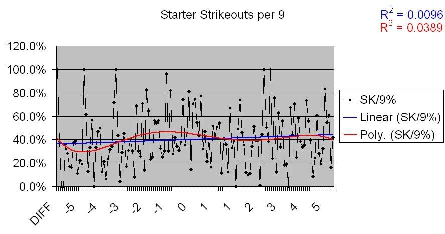
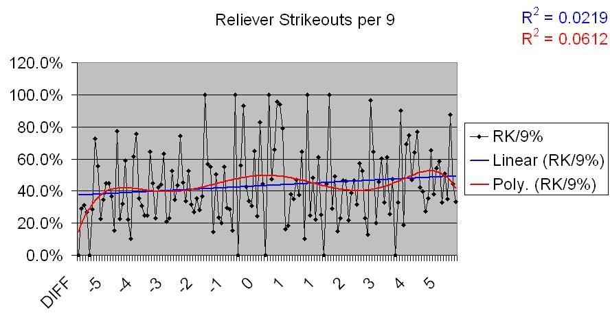
So, not much of a correlation there. That makes sense given what we saw above regarding Runs Allowed data. So, is there a correlation for underperforming teams, as there was with Runs Allowed?
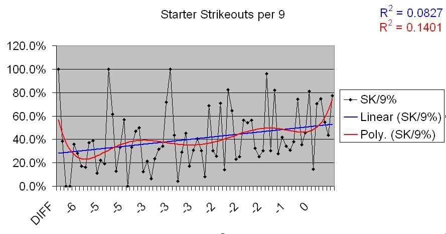
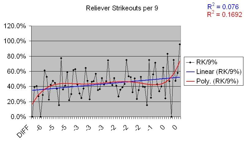
There certainly seems to be. There’s a lot of deviation there, but there’s also a pretty noticeable trend.
Let’s run these charts for two other pitching stats; ERA and OPS Allowed.
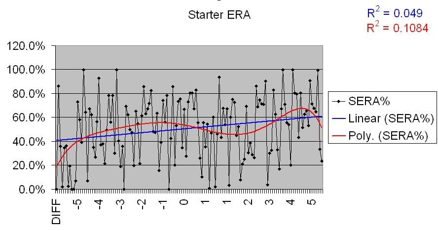
Starter ERA for overperforming teams:
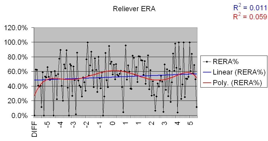
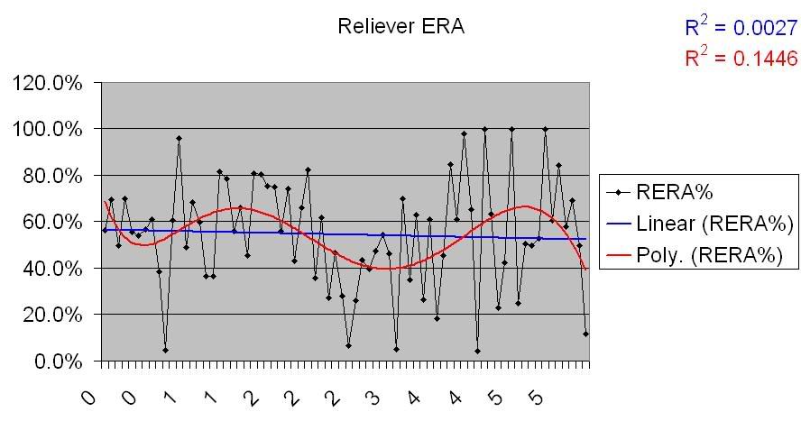
Reliever ERA for overperforming teams:
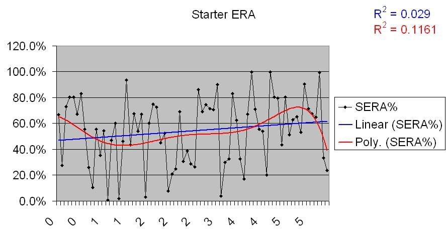
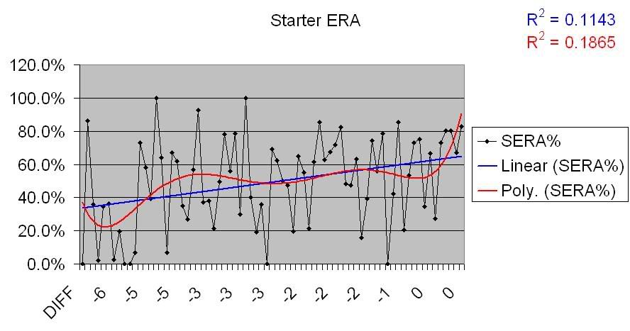
Starter ERA for underperforming teams:
Reliever ERA for underperforming teams:
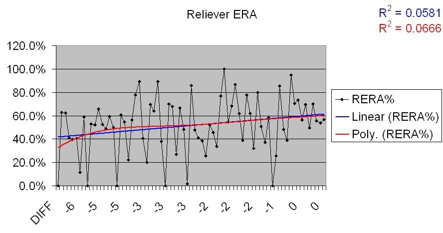
Same deal. Definite though somewhat deviant positive correlation for underperforming teams, no correlation for overperforming teams. I won’t post the charts, because they show the same basic thing, but here are links for the OPSA graphs:
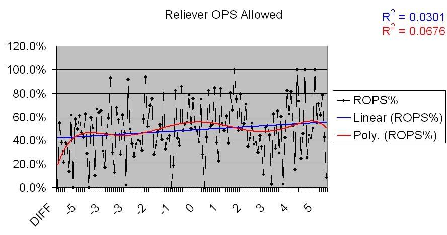
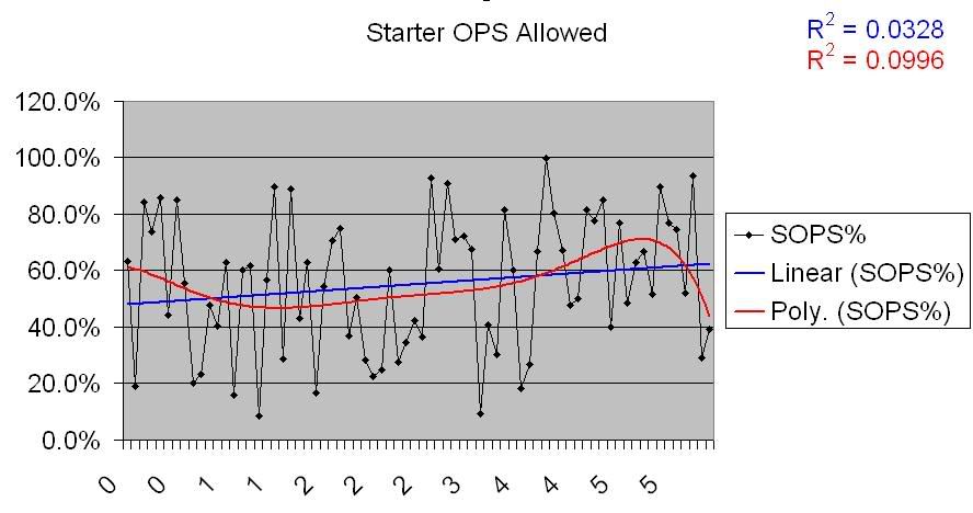
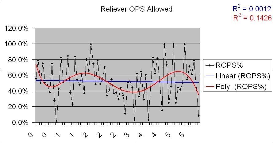
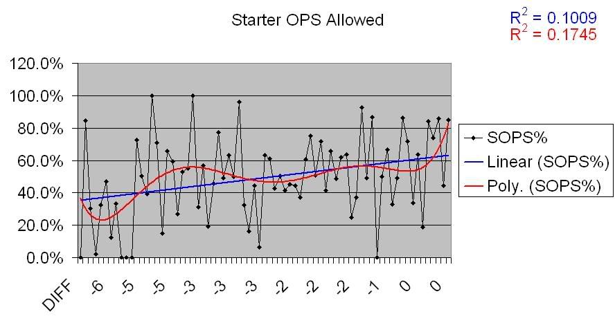
Starter OPSA
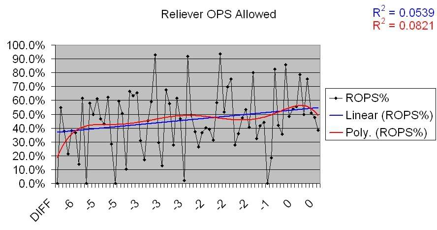
Reliever OPSA
Starter OPSA on overperforming teams
Reliever OPSA on overperforming teams
Starter OPSA on underperforming teams
Reliever OPSA on underperforming teams
Conclusions
So, that’s all he hard data. What has it told us?
I can see two definite conclusions here, and they’re inter-related. First, the only aspect of a team’s performance that seems to impact the Pythagorean differential in any consistent way is pitching. We saw it in the Runs Allowed data, and in ERA, OPS, and
Add The Sports Daily to your Google News Feed!